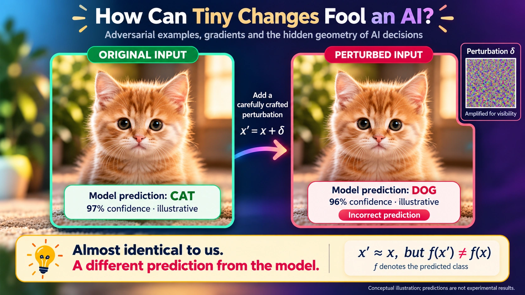
Back to blog The Learning Studio Blog

How Can Tiny ChangesFool an AI?

Adversarial Examples, Gradients and the Hidden Geometry of AI Decisions

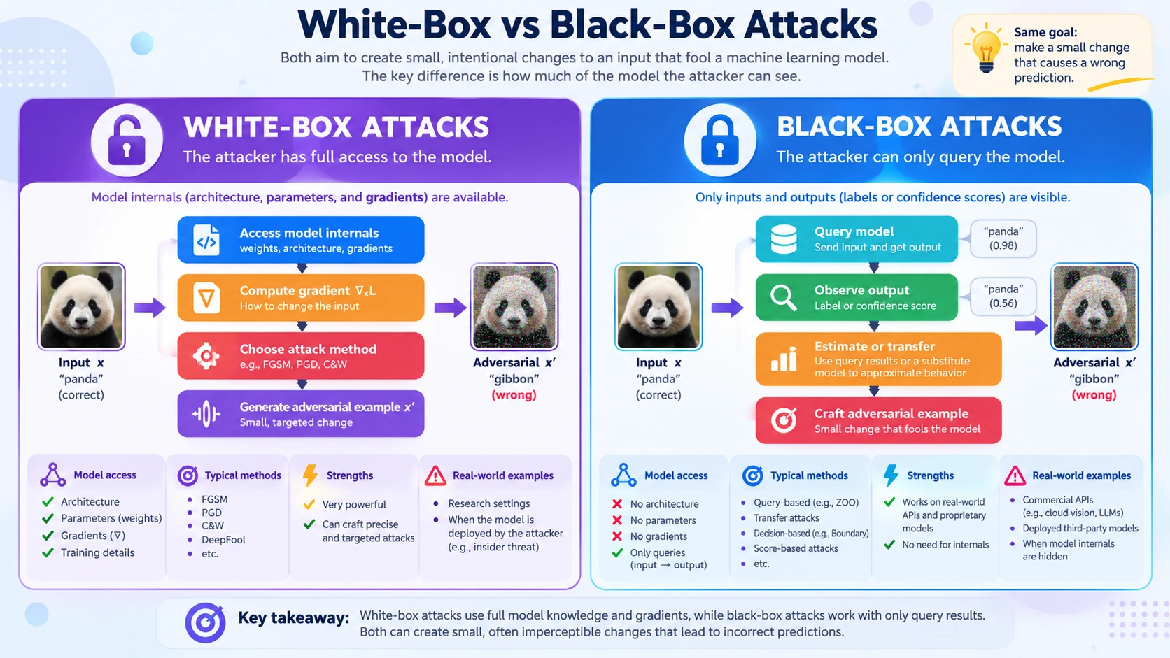
Two images can look almost identical to us. Yet an AI model might classify the first as Cat - 97% confidence and the second as Dog - 96% confidence.

What changed? Possibly only a tiny pattern of pixel-level changes. The image looks the same. The prediction does not. Why? Because underneath the image lies mathematics.

The AI Does Not See a Cat

Humans see eyes, ears, whiskers and fur, and immediately think: Cat. A neural network receives numbers. An image can be represented as a vector:

x = [x_1, x_2, \ldots, x_n]

So the model is really processing a point in a very high-dimensional space.

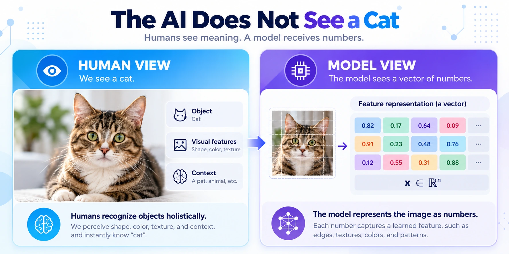
Human view of a cat compared with a model view that represents image pixels and features as a vector of numbers.

That matters because the model divides this space into regions. One region may correspond to Cat, another to Dog, and another to Bird. The boundaries between these regions are called decision boundaries.

A Tiny Move Can Change the Decision

Suppose the model predicts:

f(x) = \mathrm{Cat}

Now add a tiny perturbation, $\delta$ :

x' = x + \delta

If $\delta$ is very small, then visually $x' \approx x$ . But if that small change pushes the input across a decision boundary:

f(x') \ne f(x)

The model may suddenly predict Dog.

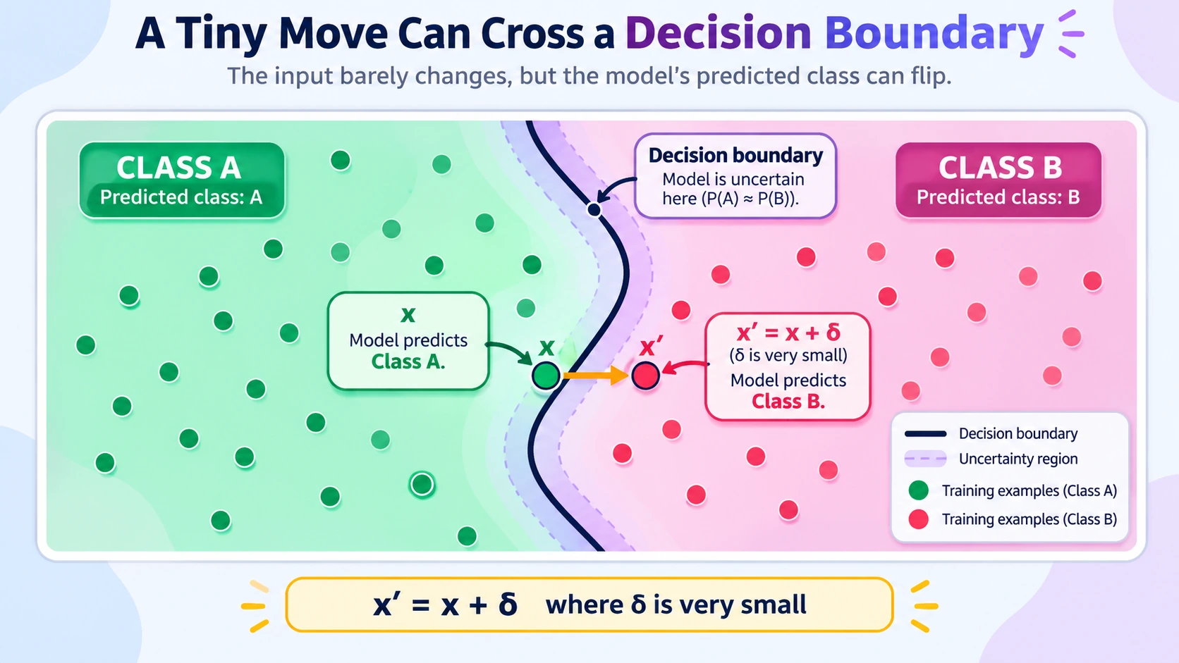
A small perturbation moves an input from the Class A region across a decision boundary into the Class B region.

The important point is this: the image does not need to change much. It only needs to move in the right mathematical direction.

So How Do We Find That Direction?

This is where gradients enter. During training, gradients help us answer: “Which direction should we change the model to reduce the loss?”

For an adversarial attack, we reverse the question: “Which direction should we change the input to increase the loss?”

If the loss is $L(x, y)$ , then the gradient with respect to the input,

\nabla_x L(x, y),

tells us how sensitive the loss is to changes in the input. You can think of it as a vulnerability map.

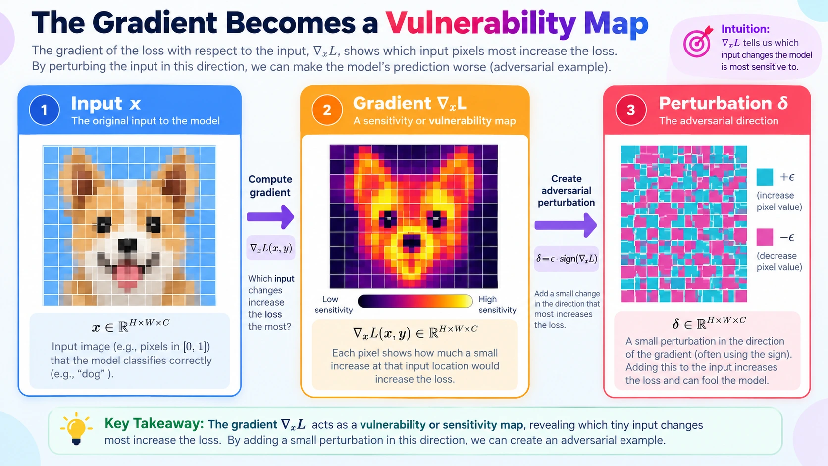
An input image, a gradient sensitivity map, and a perturbation illustrate how gradients identify directions that increase the loss.

Some tiny changes barely matter. Others matter a lot. The gradient points toward the sensitive directions.

The Fast Gradient Sign Method

One famous adversarial method is FGSM - Fast Gradient Sign Method. Its idea is:

x' = x + \varepsilon \cdot \operatorname{sign}\!\left(\nabla_x L(x, y)\right)

Here:

$x$ is the original input.
$\nabla_x L(x, y)$ is the gradient of the loss with respect to the input.
$\operatorname{sign}(\nabla_x L(x, y))$ gives the coordinate-wise direction of change.
$\varepsilon$ controls how large the perturbation is allowed to be in each coordinate.

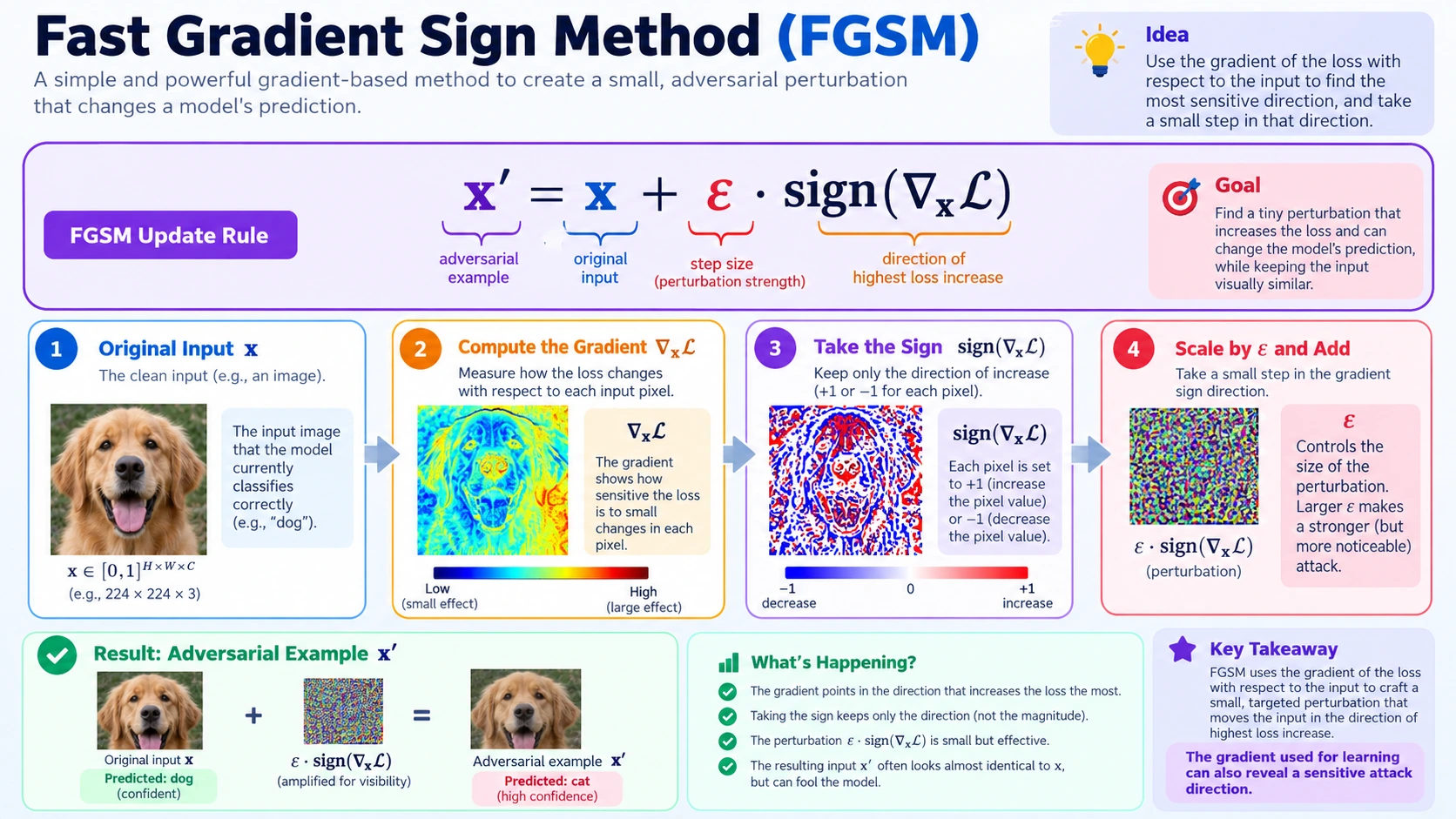
FGSM workflow: start with an image, compute the loss gradient, take its sign, scale it by epsilon, and add the perturbation to the input.

So the attack is not randomly changing pixels. It is using calculus. The same gradient that helps a model learn can also reveal where the model is fragile.

Why Can Tiny Changes Add Up?

Modern AI models work in very high-dimensional spaces. Suppose a simplified model score is:

z = w \cdot x + b

Now perturb the input to $x' = x + \delta$ . Then the score changes by:

\Delta z = w \cdot \delta = \sum_{i=1}^{n} w_i\delta_i

Each individual $\delta_i$ may be tiny. But there may be thousands or millions of them. Small changes can add up.

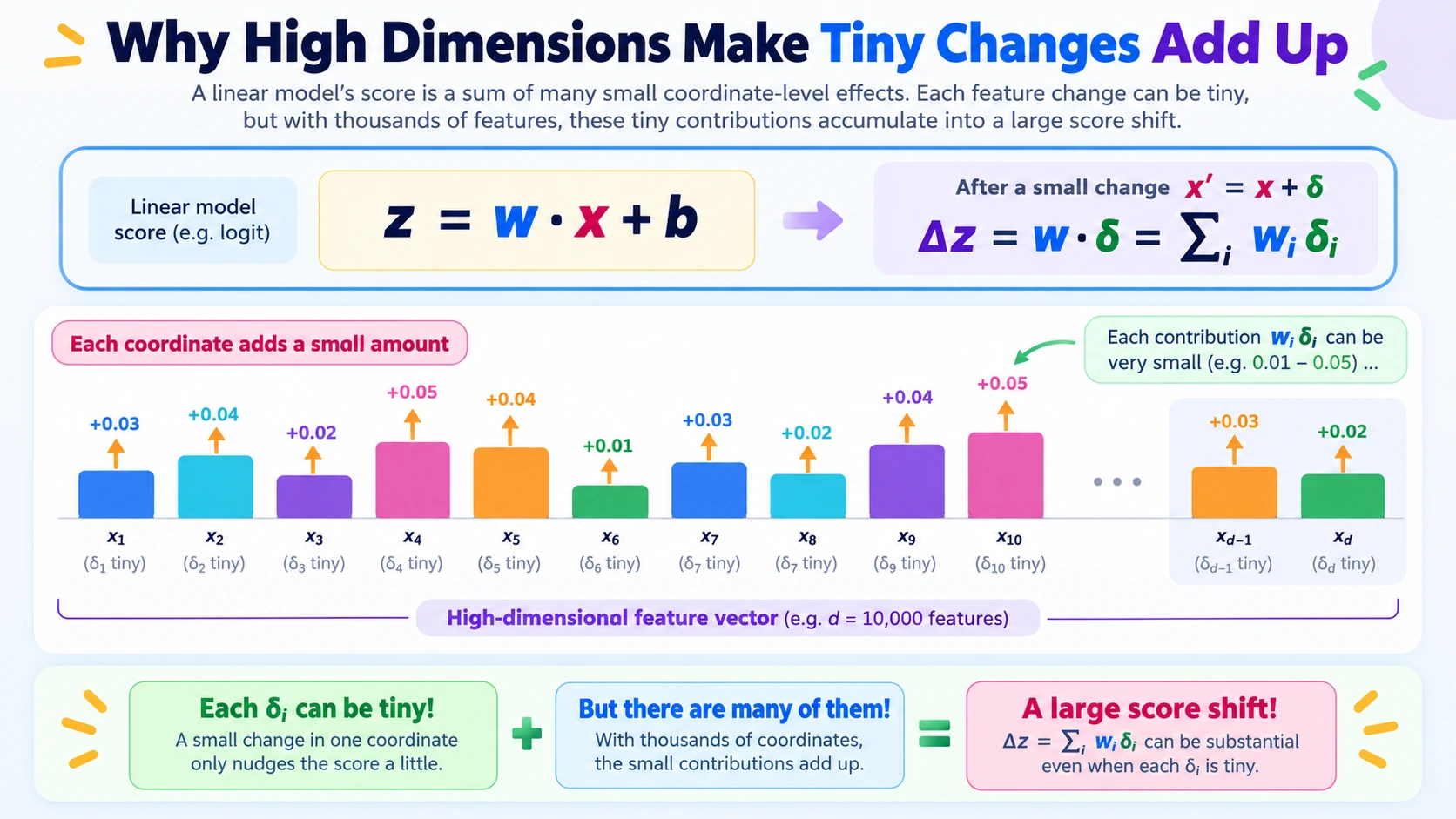
Many small coordinate-wise contributions accumulate in a linear model, producing a large change in its score in high dimensions.

This is one reason adversarial examples can be so effective. Humans barely notice the visual difference, while the model’s internal score may change substantially.

What Does “Tiny” Mean?

Even the word tiny needs mathematics. Different attacks use different measures:

$L_0$ -style measure: How many coordinates changed?
$L_2$ distance: How large is the overall Euclidean change?
$L_\infty$ distance: What is the largest change to any one coordinate?

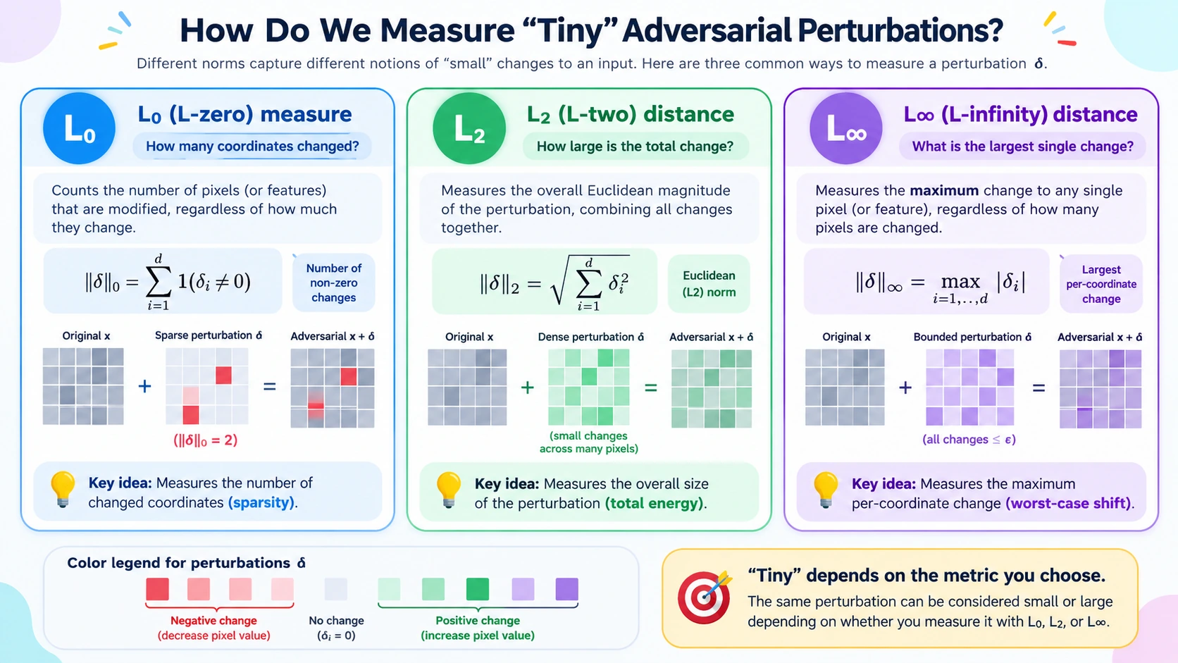
Comparison of L-zero, L-two, and L-infinity perturbation measures: number of changed coordinates, overall Euclidean change, and largest coordinate change.

So two images may be close under one measure and less close under another. Even similarity has a mathematical definition.

Confidence Can Flip Too

The model may not only change its answer. It may do so with high confidence. For example: before, Cat - 97%; after, Dog - 96%.

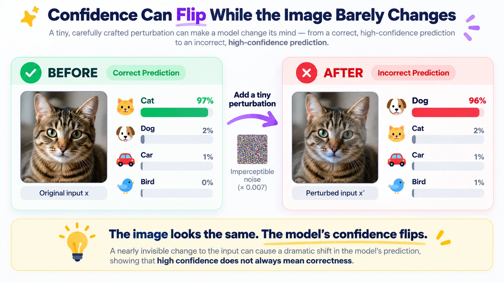
Illustrative before-and-after predictions show a nearly unchanged cat image switching from cat at 97 percent confidence to dog at 96 percent confidence.

This reinforces an important idea: confidence does not guarantee correctness. A model can be very confident and still be wrong.

Can We Make AI More Robust?

One approach is adversarial training. During training, we deliberately show the model difficult perturbed inputs. The attacker tries to maximize the loss, while the model tries to minimize the loss.

This becomes a min-max optimization problem. Conceptually:

\min_{\theta}\;\mathbb{E}_{(x,y)}\!\left[ \max_{\lVert\delta\rVert \le \varepsilon} L(\theta, x + \delta, y) \right]

Here, $\theta$ represents the model parameters, and $\lVert\delta\rVert \le \varepsilon$ limits the allowed perturbation. The goal is simple: make the model less sensitive to tiny worst-case changes.

White-box attacks use access to model internals and gradients, while black-box attacks rely on querying a model and observing its outputs. — Attack settings differ: white-box attacks have access to model internals; black-box attacks work from observed outputs.

The Bigger Idea

At first, the mystery was: “How can changing a few pixels fool an AI?” But the deeper question is: “Why can a tiny movement in input space produce such a large change in decision space?”

The answer involves vectors, decision boundaries, gradients, optimization and high-dimensional geometry. Adversarial examples remind us that AI does not reason about images the way humans do. It operates through mathematical structure.

The Takeaway

An adversarial example starts with $x$ , then adds a small perturbation:

x' = x + \delta

The change may be almost invisible to us. But if it moves the input across a decision boundary, the prediction may change dramatically.

The main lesson goes beyond “AI can be fooled”: AI decisions live inside a mathematical geometry that may behave very differently from human intuition. Once we understand the geometry, the strange behaviour begins to make sense.

Learning with Purpose

At The Learning Studio, I find topics like this especially useful because they begin with surprise. Two images look the same. The AI gives two completely different answers. Then we unpack the mathematics:

Image → Numbers → Vectors → Geometry → Gradients → Optimization

And suddenly the mystery becomes understandable. That is what makes AI mathematics so fascinating.

Coming Next

How Does AI Decide What to Pay Attention To?

The Mathematics of Attention - Queries, Keys, Values and Dot Products

How does a model decide which words matter most? Why do dot products appear? Why are vectors called Queries, Keys and Values? And how can a compact mathematical idea become one of the foundations of modern language models?

That is where we go next.